3. Extending Recorder 6

3.1. SQL Server

3.1.1. Master Table

In order for the Data Selector tool to be able to extract species records from Recorder6 a SQL script must be run to create and update a master table in the Recorder6 database. The SQL script will be specific to your requirements based on a whole host of considerations. For example:

• Which columns/attributes to be defined in the table.

• Which surveys, events, samples and occurrences to include in the table.

• Whether any confidential surveys, species or occurrences should be included/excluded or flagged as confidential in the table.

• Whether any sensitive species should have their precision altered in the table.

• What species designations are to be included and how they should appear in the table (e.g. into which columns and using what abbreviations).

• How any occurrence abundance/counts and associated measurement qualifier/types should appear in the table.

• If zero abundance records are to be included in the table (in which case they would be clearly flagged as zero abundance).

• If a cut-off date for specific taxonomic groups or species is used to flag them as historic records.

• If the standard Recorder6 taxon group names or more bespoke group names are used (e.g. splitting ‘terrestrial mammal’ into ‘Mammals - Terrestrial (bats)’ and ‘Mammals - Terrestrial (excl. bats)’.

• Whether unverified and/or unchecked records are included in the table.

• How record dates are to appear (e.g. as vague date range or as just single dates).

• If any specific records are to be flagged (e.g. bat records containing ‘roost’ or ‘hibern’ in any record/sample comments or measurements, or bird records containing ‘breed’, ‘bred’ or ‘nest’).

Note

Multiple master SQL tables, or multiple views on the same SQL table, can be created as required.

3.1.2. Spatial Data

If your Recorder6 database is running on a more recent version of SQL Server (i.e. SQL Server 2016 or later) then it supports ‘Geometry’ and ‘Geography’ spatial data type. In this case the master table can also be ‘spatialized’ by setting the geometry for all records as points and/or polygons. This enables spatial queries to be performed within SQL Server rather than the GIS application thereby reducing the work load in GIS and utilising the likely increased performance capabilities of many servers running SQL Server.

In order to ‘spatialize’ the master table additional steps in the SQL script are run to calculate the geometry of all records based on their grid reference. The geometry can be calculated as points and/or polygons based on the requirements of the LERC and how the data will be used. Once spatialized, records from the master table can be directly plotted and viewed as points or polygons in GIS. In addition, queries can be executed in SQL Server using the spatial location of the records in much the same way that spatial queries can be performed in GIS. This reduces the overheads in GIS and means that the number of records exported from SQL Server into GIS can be much reduced.

3.2. The Data Selector tool

3.2.1. Tool components

There are four component parts to the Data Selector tool that work together to automate the process described above:

1. Spatial data held in a SQL Server database (a stored procedure for its extraction is also required).

2. A tool XML configuration file that specifies how if the user can choose a user XML profile.

3. One or more user XML profiles that specifies how the tool is set up and how data will be saved by default.

4. The Data Selector tool ArcGIS Pro add-in.

3.2.2. Tool workflow

The Data Selector tool requires minimum user input in order to perform queries once it is configured. The simple workflow is as follows (see Fig. 3.1):

1. The user lists all the attributes (columns) from the selected SQL table to return (or enters ‘*’ to return all attributes).

2. The user selects which SQL table or view to query.

3. The user specifies any ‘Where’ selection criteria, if any, to apply when selecting records from the SQL table.

4. The user also specify any ‘Group By’ and ‘Order By’ criteria to apply when selecting records from the SQL table.

5. The user selects what output format should be created for the selected records.

6. The user opts to clear the log file before use and/or open the log file after completion.

7. The user clicks Run the process starts.

Fig. 3.1 The Data Selector tool workflow

In essence, the process that the tool follows is identical to the manual process a user would perform:

1. The required columns and records from the SQL table are selected based on the specified criteria.

2. The selected records are saved to the target file in the required output format.

3. During the process the tool records its progress to a log file and, when the process finishes, this log file can be displayed to allow the user to assess the success of the data selection. The log file in a location specified in the user XM profile.

3.2.3. Tool outputs

When the process finishes, the output is added to the GIS interface, either as a new GIS layer or as a non-spatial text table.

The tool will output GIS layers as ESRI (.shp) shapefiles or as file-geodatabase feature classes. An example of the output the tool can generate is showin in Fig. 3.2.

Fig. 3.2 Example of a GIS spatial output from the Data Selector tool

Text file outputs can be generated in CSV format (Fig. 3.3) or TXT format.

Fig. 3.3 Example of a text file output from the Data Selector tool

Finally, the log file details each step that was taken during the process, and gives some feedback about the outcome of the process. This includes reporting on the chosen options for the selection, the number of records that were selected and if the output contains spatial data (Fig. 3.4).

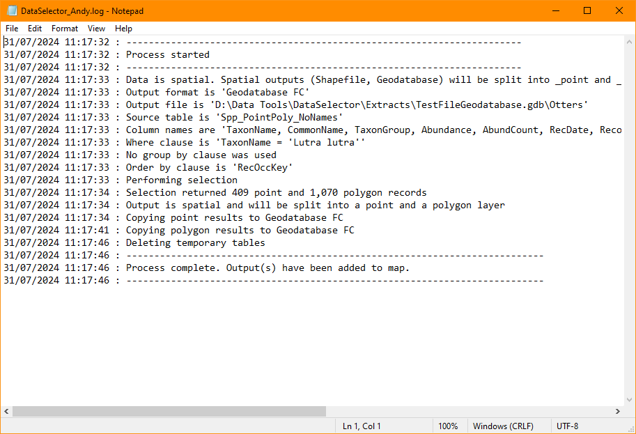
Fig. 3.4 Example of a Data Selector tool log file

The following chapters, Setting up the tool and Running the tool, will guide you through setting up and operating the tool in such a way that these tool outputs meet the general requirements of data selection within your organisation.